Clarifications
This section provides clarifications for potentially confusing usages and parameters.
Demo Model
Many clarifications are based on examples. We will use our demo model in below. You can get a copy of it by piegy.simulation.demo_model.
from piegy import simulation

mod = simulation.demo_model()
simulation.run(mod)
interval
piegy. omitted)analysis.check_convergence, test_var.var_convergence1, test_var.var_convergence2, figuresinterval essentially means: take average over some data points.
It denotes the length of a “data interval”. We take the average value over every such interval of data points, and work with these average values to smooth out local randomness.
For example, in our demo model, if we make a U, V payoff - time plot without taking any average (i.e., interval = 1), the figure is:
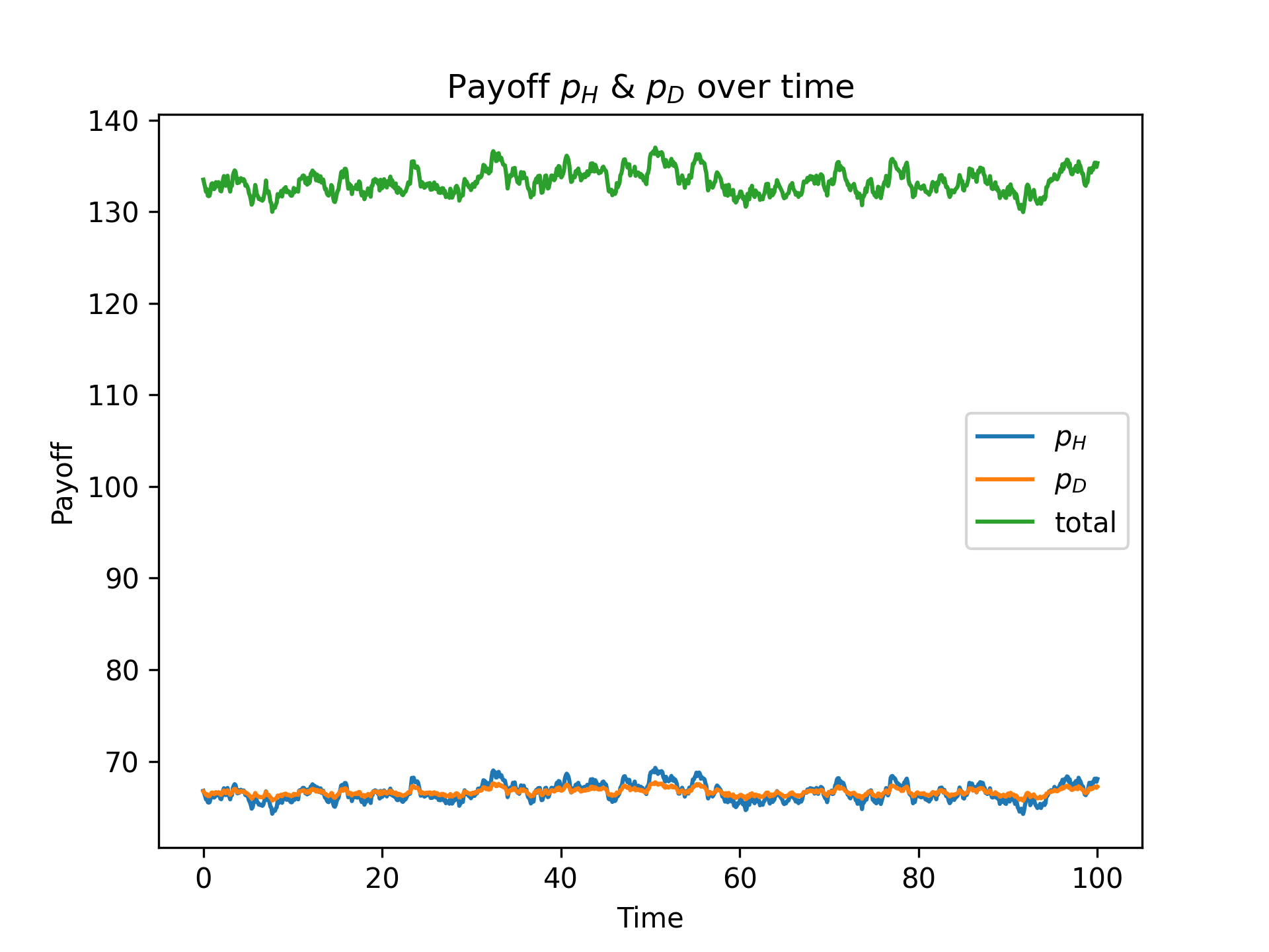
pi_dyna with interval = 1
interval, say set it to 40: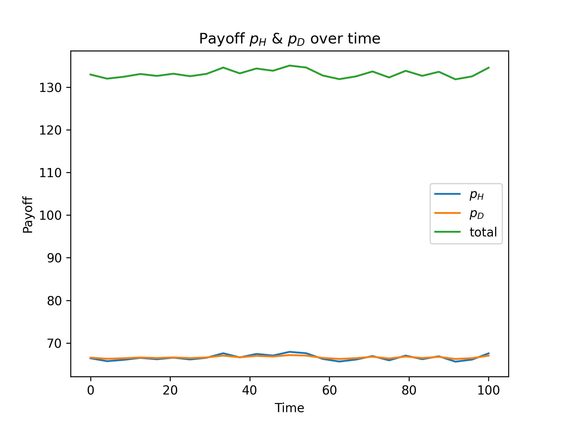
pi_dyna with interval = 40
Now it looks much cleaner. You may notice the x-range is reduced to around 80. That is exactly because we are taking averages: every 40 original data points give a new “average point”.
compress_data and compress_ratio
compress_datais a class method ofpiegy.simulation.model.compress_ratio:parameter for
compress_data.A
piegy.simulation.modelobject also hascompress_ratiohas a variable. Stores current ratio of data reduction, initialized as 1 and updated bycompress_data.
compress_data is an effort to reduce data size by saving only average values rather than every data point.
For example, let’s look at how many numbers are contained in sim (our demo model, see parameters at Typical Params)
We have
N * M * 12input parameters (initial population, matrices, patch parameters, etc.)As for the data generated during simulation, there
N * M * maxtime / record_itvfor U’s population. That is \(10 \cdot 10 \cdot 3000 = 3 \cdot 10^5\) in our case.And similarly for V population, U and V payoff.
So we will be saving about \(12 \cdot 10^6\) numbers in total — that’s a lot!
There is indeed a way to reduce data at the expense of losing accuracy: take average over every some interval of data points and save these average values. This is done by compress_data.
For example, by calling:
mod.compress_data(10)
it goes through every patch and takes average over every 10 original data points, store the average, then move on to the next 10.
The change is in-place, i.e., directly modifies sim.
Then for mod.U (U population), we used to store 10 * 10 * 3000 values, and now its size is reduced to 10 * 10 * 300.
In terms of the total number of data points, we only need to save \(12 \cdot 10^5\) numbers now, reduced by 10 times.
However, the actual size shown in file system is probably not divided by 10. That may be due to some json behaviors (data are stored in json format).
The size reduction comes at the expense of:
The original data are lost; we only have average values now.
The new data become coarser as we use larger
compress_ratio.
You can call compress_data repeatedly, and data will become coarser and coarser as well. For example, calling mod.compress_data(10) again takes average over every \(10 \cdot 10\) points; essentially the same as mod.compress_data(100).
You can check the current reduction ratio by printing out compress_ratio variable of sim:
print(mod.compress_ratio)
Considerations regarding interval and compress_ratio
Here
intervalrefers to parameters of functions inpiegy.figures,piegy.analysis,piegy.test_var.compress_ratiorefers to variable of apiegy.simulation.modelobject, which records ratio of data reduction.
There might be considerations whether interval and compress_ratio would have conflicts. The answer is No.
Our codes are specifically designed to accommodate both two intervals, in the following way:
Say
interval = 10.If
compress_ratiois 1, then make plots / perform other analysis as they were: take average over every 10 data points and proceed.If
compress_ratiois not 1, scaleintervalby:interval = int(interval / compress_ratio)
and then proceed. So that we will still be taking average over the same number of data points (in terms of the original data).
If
compress_ratiois larger thaninterval, the above code would result in the newintervalbeing 0. We then set it to 1 and print a warning message: data is coarser than the expected interval.
start and end
piegy. omitted)analysis.check_convergence, figures, test_varstart and end parameters point to some proportion of maxtime.start being the lower bound and end being upper bound.maxtime = 300 in the our demo model, start = 0.9 points to the time point at 300 * 0.9 = 270, and end = 1.0 points to 300 * 1.0 = 300.start and end, essentially the last 10% of time.Convergence and fluc
fluc is a param in: (piegy. omitted)analysis.check_convergence, test_var.var_convergence1, test_var.var_convergence2fluc threshold.For U population:
Get average data based on the
intervalparam (all 3 functions have this paramter).Get the max and min of the average data.
Fluctuation of U is then given by \(\frac{(max - min)}{min}\). Similarly for V.
Consider the result convergent if both fluctuations are less than
fluc.