piegy.test_var

This module contains tools to test the influence of one or two patch variables on the simulation results.

Test Functions

The two functions below perform tests on one or two patch variables and save data.

Intended to combine with the plot functions in this module to visualize the results.

test_var.test_var1(mod, var, values, dirs, compress_ratio=1, scale_maxtime=False)

Test the influence of one patch variable on simulation results.

test_var1 makes copies of mod and changes the patch variable var to the specified values (in all patches), perform simulations, and then save data. The original mod is not changed.

Parameters:

• mod (piegy.simulation.model object) – where the parameters of the model and data are stored.

• var (str) – which variable to test. Expect a string of the variable name, such as 'mu1', 'kappa1'.

• values (list or numpy.ndarray) – what values of var to test.

• dirs (str) – where to save test data. Expect a path to a folder. test_var1 then create subfolders inside dirs and store data.

• compress_ratio (int) – used to reduce data size: takes average over every 'compress_ratio' many data points when saving. Passed to piegy.simulation.model.compress_data method.

• scale_maxtime (bool) – whether to scale maxtime of tests towards the input mod. Intended to avoid unnecessarily long runtime possibly encountered in tests due to different values.

Returns:

a list of directories where all test results are stored. One directory corresponds to one value of var.

Return type:

list of str

test_var.test_var2(mod, var1, var2, values1, values2, dirs, compress_ratio=1, scale_maxtime=False)

Test the influence of two patch variables on simulation results.

Note which variable comes first does make a difference when plotting: var2 will be placed on x-axis, while different values of var1 are represented by different curves.

test_var2 makes copies of mod and changes the patch variables var1 and var2 to the specified values (in all patches), perform simulations, and then save data. The original mod is not changed.

Parameters:

• mod (piegy.simulation.model object) – where the parameters of the model and data are stored.

• var1 (str) – the first variable to test. Expect a string of the variable name, such as 'mu1', 'kappa1'.

• var2 (str) – the second variable to test.

• values1 (list or numpy.ndarray) – what values of var1 to test.

• values2 (list or numpy.ndarray) – what values of var2 to test.

• dirs (str) – where to save test data. Expect path to a folder. test_var2 then create subfolders inside dirs and store data.

• compress_ratio (int) – used to reduce data size: takes average over every 'compress_ratio' many data points when saving. Passed to piegy.simulation.model.compress_data method.

• scale_maxtime (bool) – whether to scale maxtime of tests towards the input mod. Intended to avoid unnecessarily long runtime possibly encountered in tests due to different values.

Returns:

a 2D list of directories where all test results are stored. One directory corresponds to one pair of var1 value and var2 value.

Return type:

2D list of str

Plot Functions

The following functions help to visualize simulation results.

test_var.var_HV1(var, values, var_dirs, ax_H=None, ax_D=None, start=0.95, end=1.0, color_H='purple', color_D='green')

Plots how U, V average population over a specified time interval change with different values of a patch variable.

Parameters:

• var (str) – which patch variable you tested. Expect a string of the variable name, such as 'mu1', 'kappa1'.

• values (list or numpy.ndarray) – what values you tested with.

• var_dirs (list of str) – where test results are stored. Expect the return value of piegy.test_var.test_var1. You can get a copy of it by piegy.test_var.get_dirs1 if lost. Data not existing are ignored.

• ax_H (matplotlib axes) – matplotlib axes to plot the change of U population over values. A new axes will be created if None is given.

• ax_H – matplotlib axes to plot the change of V population over values. A new axes will be created if None is given.

• start (float) – lower bound of the time interval to plot.

• end (float) – upper bound of the time interval to plot. For details of start and end, see Clarifications-start_end.

Returns:

two figures of how U, V population change with values of var

Return type:

matplotlib figures.

test_var.var_HV2(var1, var2, values1, values2, var_dirs, ax_H=None, ax_D=None, start=0.95, end=1.0, color_H='viridis', color_D='viridis', alpha=1)

Plot how U, V average population over a specified time interval change with different values of two patch variables.

var2 values are shown on the x-axis; var1 values are shown by different curves.

Parameters:

• var1 (str) – the first patch variable you tested. Expect a string of the variable name, such as 'mu1', 'kappa1'.

• var2 (str) – the second patch variable you tested.

• values1 (list or numpy.ndarray) – what values for var1 you tested.

• values2 (list or numpy.ndarray) – what values for var2 you tested.

• var_dirs (double list of str) – where test results are stored. Expect the return value of piegy.test_var.test_var2. You can get a copy of it by piegy.test_var.get_dirs2 if lost. Data not existing are ignored.

• ax_H (matplotlib axes) – matplotlib axes to plot the change of U population over values1 and values2. A new axes will be created if None is given.

• ax_H – matplotlib axes to plot the change of V population over values1 and values2. A new axes will be created if None is given.

• start (float) – lower bound of the time interval to plot.

• end (float) – upper bound of the time interval to plot. For details of start and end, see Clarifications-start_end.

• color (str) – used to set gradient colors for the curves in plots. Expect name of a matplotlib color map.

• alpha (float) – alpha value of the color RGB params. Used to make points semi-transarent if overlapping.

Returns:

two figures of how U, V payoff change with values of var1 and var2

Return type:

matplotlib figures.

test_var.var_pi1(var, values, var_dirs, ax_H=None, ax_D=None, start=0.95, end=1.0, color_H='violet', color_D='yellowgreen')

Plots how U, V average payoff over a specified time interval change with different values of a patch variable.

Parameters:

• var (str) – which patch variable you tested. Expect a string of the variable name, such as 'mu1', 'kappa1'.

• values (list or numpy.ndarray) – what values you tested with.

• var_dirs (list of str) – where test results are stored. Expect the return value of piegy.test_var.test_var1. You can get a copy of it by piegy.test_var.get_dirs1 if lost. Data not existing are ignored.

• ax_H (matplotlib axes) – matplotlib axes to plot the change of U payoff over values. A new axes will be created if None is given.

• ax_H – matplotlib axes to plot the change of V payoff over values. A new axes will be created if None is given.

• start (float) – lower bound of the time interval to plot.

• end (float) – upper bound of the time interval to plot. For details of start and end, see Clarifications-start_end.

Returns:

two figures of how U, V payoff change with values of var

Return type:

matplotlib figures.

test_var.var_pi2(var1, var2, values1, values2, var_dirs, ax_H=None, ax_D=None, start=0.95, end=1.0, color_H='viridis', color_D='viridis', alpha=1)

Plot how U, V average payoff over a specified time interval change with different values of two patch variables.

var2 values are shown on the x-axis; var1 values are shown by different curves.

Parameters:

• var1 (str) – the first patch variable you tested. Expect a string of the variable name, such as 'mu1', 'kappa1'.

• var2 (str) – the second patch variable you tested.

• values1 (list or numpy.ndarray) – what values for var1 you tested.

• values2 (list or numpy.ndarray) – what values for var2 you tested.

• var_dirs (double list of str) – where test results are stored. Expect the return value of piegy.test_var.test_var2. You can get a copy of it by piegy.test_var.get_dirs2 if lost. Data not existing are ignored.

• ax_H (matplotlib axes) – matplotlib axes to plot the change of U payoff over values1 and values2. A new axes will be created if None is given.

• ax_H – matplotlib axes to plot the change of V payoff over values1 and values2. A new axes will be created if None is given.

• start (float) – lower bound of the time interval to plot.

• end (float) – upper bound of the time interval to plot. For details of start and end, see Clarifications-start_end.

• color (str) – used to set gradient colors for the curves in plots. Expect name of a matplotlib color map.

• alpha (float) – alpha value of the color RGB params. Used to make points semi-transarent if overlapping.

Returns:

two figures of how U, V payoff change with values of var1 and var2

Return type:

matplotlib figures.

Other Functions

Other useful functions.

test_var.var_convergence1(var_dirs, interval=20, start=0.75, fluc=0.05)

Check whether the test results converge, used when just one variable is tested. This function calls check_convergence function in piegy.simulation_analysis.

Please use piegy.test_var.var_convergence2 to check convergence when testing two vairables.

Parameters:

• var_dirs (double list of str) – where all test results are stored. Expect the return value of piegy.test_var.test_var1. You can get a copy of it by piegy.test_var.get_dirs1 if lost. Data not existing are ignored.

• interval (int) – takes average over some number of data points to smooth data.

• start (float) – defines a time point. Calculate fluctuation of U, V population after this point.

• fluc (float) – threshold of fluctuation. Check whether max fluctuation of U, V population after start proportion of time is less than this threshold.

Returns:

a list of directories where the data didn’t converge.

Return type:

list of str

test_var.var_convergence2(var_dirs, interval=20, start=0.75, fluc=0.05)

Check whether the test results converge, used when just one variable is tested. This function calls check_convergence function in piegy.simulation_analysis.

Please use piegy.test_var.var_convergence2 to check convergence when testing two vairables.

Parameters:

• var_dirs (double list of str) – where all test results are stored. Expect the return value of piegy.test_var.test_var2. You can get a copy of it by piegy.test_var.get_dirs2 if lost. Data not existing are ignored.

• interval (int) – takes average over some number of data points to smooth data.

• start (float) – defines a time point. Calculate fluctuation of U, V population after this point.

• fluc (float) – threshold of fluctuation. Check whether max fluctuation of U, V population after start proportion of time is less than this threshold.

Returns:

a list of directories where the data didn’t converge.

Return type:

list of str

test_var.get_dirs1(var, values, dirs)

Mimics the format of how piegy.test_var.test_var1 creates directories and return a copy of its return value.

Used to retrieve the directories of data.

Parameters:

• var – the patch variable you tested.

• values1 (list or numpy.ndarray) – what values for var you tested.

• dirs (str) – the path of directory which you passed to test_var1 (or a new path if you re-named or moved it).

Returns:

a list of where piegy.test_var.test_var1 saved data.

Return type:

list of str

test_var.get_dirs2(var1, var2, values1, values2, dirs)

Mimics the format of how piegy.test_var.test_var2 creates directories and return a copy of its return value.

Used to retrieve the directories of data.

Parameters:

• var1 (str) – the first patch variable you tested.

• var2 (str) – the second patch variable you tested.

• values1 (list or numpy.ndarray) – what values for var1 you tested.

• values2 (list or numpy.ndarray) – what values for var2 you tested.

• dirs (str) – the path of directory which you passed to test_var2 (or a new path if you re-named or moved it).

Returns:

a double list of where piegy.test_var.test_var2 saved data.

Return type:

double list of str

Examples

The piegy.test_var module provided several handy tools to test how patch vairables influence simulation results, either population or payoff.

First please import necessary modules:

from piegy import simulation, test_var

We will use our classical demo model. You can obtain a copy by piegy.simulation.demo_model:

mod = simulation.demo_model()

If we run this demo model directly, The equilibrium U, V population is around 5.7 and 2.7 per patch. (For model parameters and simulation results, see Typical Params)

You might be wondering, would change of patch variables influence equilibrium population? If we keep all other parameters the same and change the value of just one patch variable, will the equilibrium population and payoff be different?

Great question! This is exactly what this module is made for: test infleunce of one or two patch variables on simulation results. Let’s see how to use it.

Say you want to test the mu1 variable on a few values [0.1, 0.3, 0.5, 0.7, 0.9]:

var = 'mu1'
values = [0.1, 0.3, 0.5, 0.7, 0.9]

Then you can call piegy.test_var.test_var1 to test how the above values for w1 influence population and payoff. dirs is the directory where data will be saved. The directory will be created if not existing.

dirs = 'test_var_dirs'
var_dirs = test_var.test_var1(mod, var, values, dirs)

The return value var_dirs is a list of directories where data are stored. It is structured in a fixed format and tells other functions where to find data. If you print var_dirs, it looks like:

print(var_dirs)

outputs:

['test_var_dirs/mu1=0.1', 'test_var_dirs/mu1=0.3', 'test_var_dirs/mu1=0.5',
 'test_var_dirs/mu1=0.7', 'test_var_dirs/mu1=0.9']

There are many ways to analyze data, you can either use the figure functions in piegy.figures, implement your own methods, … But piegy.test_var module does provide several handy tools. For example, let’s try test_var.var_HV1:

fig_UV, ax_UV = plt.subplots(2, 1, figsize = (6.4, 9.6))
test_var.var_HV1(var, values, var_dirs, ax_UV[0], ax_UV[1])

This function plots how U, V equilibrium population change with values of mu1:

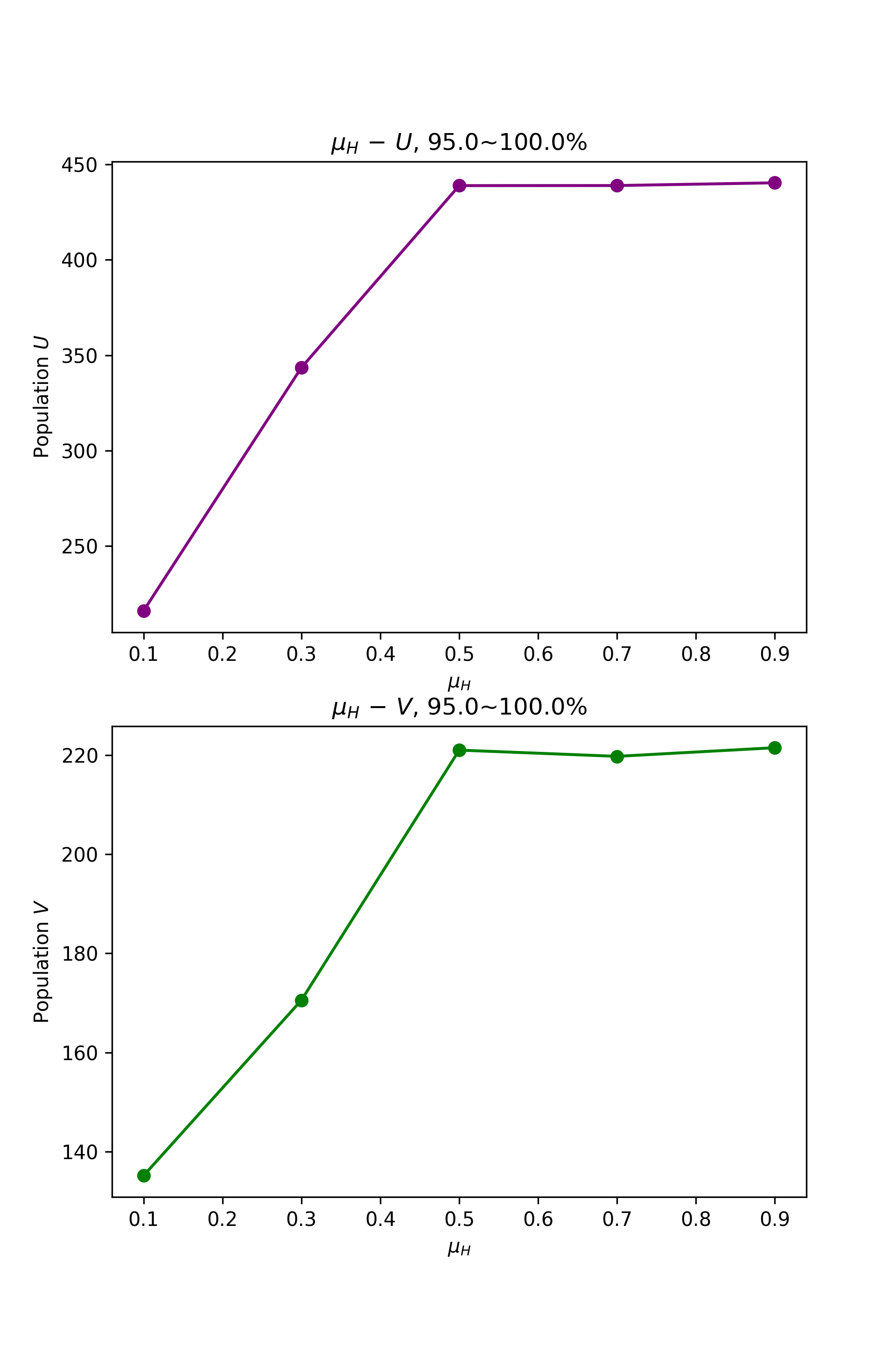
Change of U and V Population with mu1

You can also plot change of payoff by test_var.var_pi1:

fig_pi, ax_pi = plt.subplots(2, 1, figsize = (6.4, 9.6))
test_var.var_pi1(var, values, var_dirs, ax_pi[0], ax_pi[1])

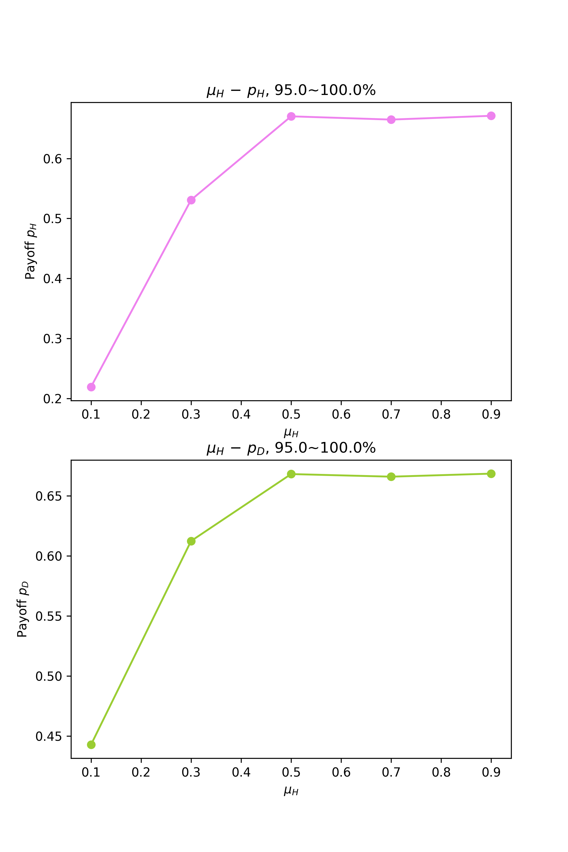
Change of U and V Payoff with mu1

We observe a roughly decreasing trend here: larger mu1 value tends to decrease population and payoff. It’s also noteworthy that our demo model mod runs the simulation only once: mod.sim_time = 1. So the figures above are probably far from accurate. If we set mod.sim_time to 20 and try more values of mu1, we could see a clearer trend.

Note all the plot functions above requires var_dirs (return value of test_var.var_HV1): it tells the functions where to find data. If you want to read from an old set of test_var1 data but don’t have the old var_dirs anymore, you can remake it by test_var.get_dirs1 function.

test_var.get_dirs1 automatically makes var_dirs based on what variable, values and the “base directory” dirs you used. You can also pass in more a larger list of values if you ran more tests afterwards.

var_dirs_remade = test_var.get_dirs1(var, values, dirs)

var_dirs_remade will be the same as the original var_dirs. You can pass it to the plot functions above.

So far we have introduced most of the test_var functions for the 1-variable tests. You can also perform 2-variable tests with the counterparts of these functions; the usage is very similar.