Typical Parameters

This section includes some typical parameters we used for simulation. They are just for reference and to get you started — try anything!

Parameters in Demo Model

Most of the examples in our piegy documentation use the same model. We list out its parameters here.

You can also get a copy of it rather conveniently by piegy.simulation.demo_model function.

from piegy import simluation  # import it if you haven't

N = 10                  # Number of rows
M = 10                  # Number of cols
maxtime = 100           # how long you want the model to run
record_itv = 0.1        # how often to record data.
sim_time = 1            # repeat simulation to reduce randomness
boundary = True         # boundary condition.

# initial population for the N x M patches.
init_popu = [[[200, 100] for _ in range(M)] for _ in range(N)]

# flattened payoff matrices
matrices = [[[-1, 4, 0, 2] for _ in range(M)] for _ in range(N)]

# patch parameters
patch_params = [[[1, 1, 10, 10, 0.001, 0.001] for _ in range(M)] for _ in range(N)]

print_pct = 50           # print progress
seed = 36               # seed for random number generation

# create a model object
mod = simulation.model(N, M, maxtime, record_itv, sim_time, boundary, init_popu, matrices, patch_params, print_pct, seed)

Quick look of population dynamics and final distribution:

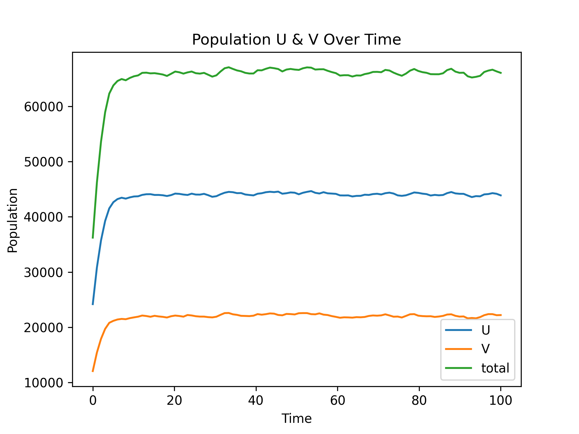
Population Dynamics

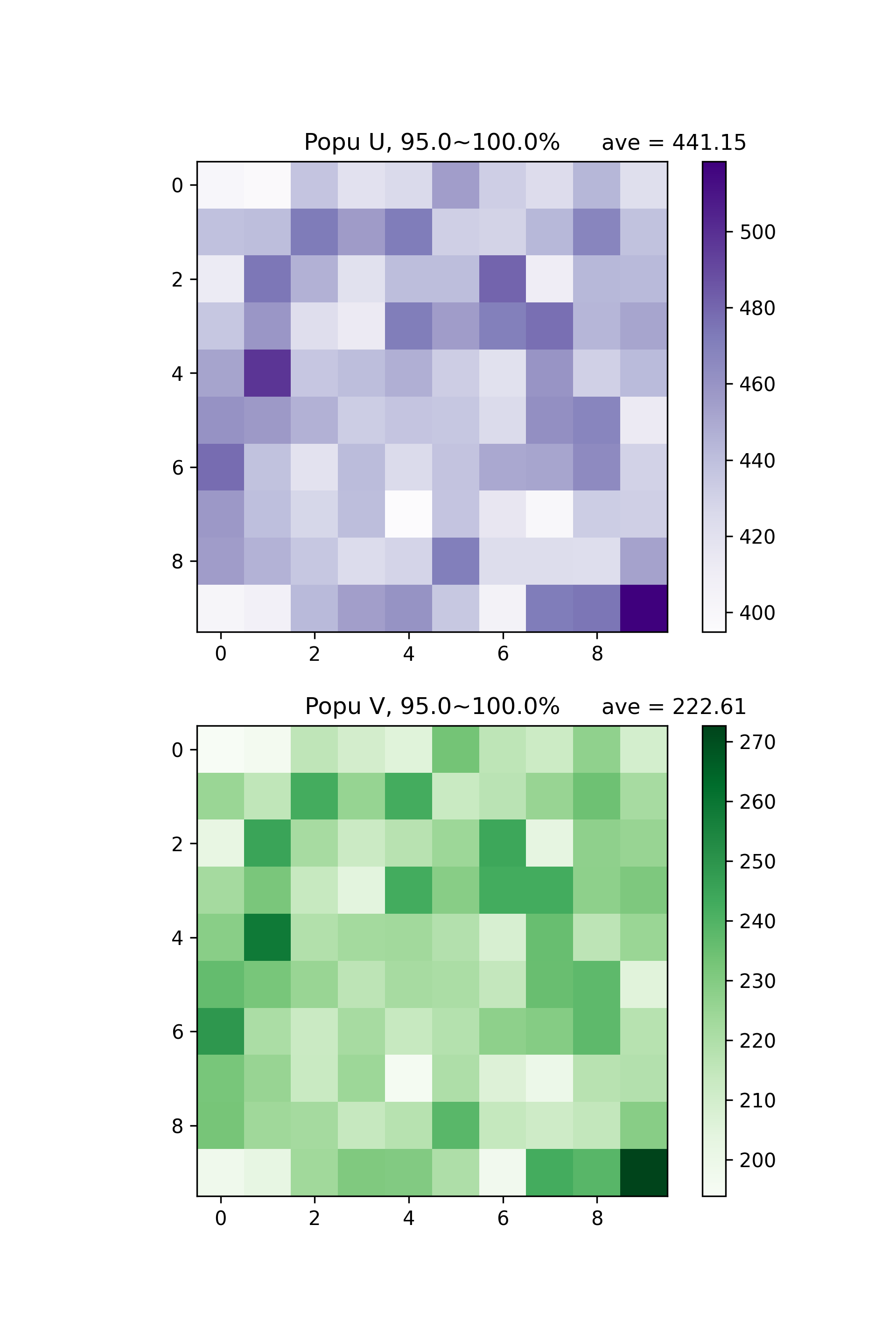
Final Distribution of U and V Population

This model has the following properties:

1. The 10 x 10 spatial dimension is large enough for sufficient migration but not exceedingly large in terms of runtime.

2. The uniform payoff matrices follow a classical predator-prey setting:

   • The cost of fighting among predators is 1

   • The total resource is 4

   • Two predators fight and each gain -1 payoff.

   • Predator eats prey and gain 0.4 payoff, while prey gain 0 payoff.

   • Preys share the resource equally and each gain 2 payoff.

3. The expected equilibrium state is 444 hawks and 222 doves at each patch, assuming no migration and stochasticity.

4. It demonstrates some interesting phenomena:

   • In terms of distribution, the model starts from uniform state but ended with a highly clustering distribution.

   • As for population, the actual equilibrium population is much smaller than expected (444, 222 per patch).

However, you may notice we run the simulation only once (sim_time = 1), and this may result in high randomness. That’s absolutely correct. For real simulations, we recommend repeat the simulation and check the final distribution.